
Despite the central role of optimization in deep learning, most optimizers rely on update structures whose functional form is fixed before training begins. This static design can limit their ability to respond to changing gradient behavior across the loss landscape, where training may shift between stable, noisy, and inconsistent regimes.
This study proposes PILOT (Policy-Informed Learned OpTimizer), an online optimizer that adapts its update behavior during training. Rather than using a fixed balance between momentum, normalization, and sign-based updates, PILOT uses gradient-direction agreement as a signal of local training stability. Conditioning the update rule on this agreement signal allows the optimizer to adjust its behavior when gradients become stable, noisy, or inconsistent.
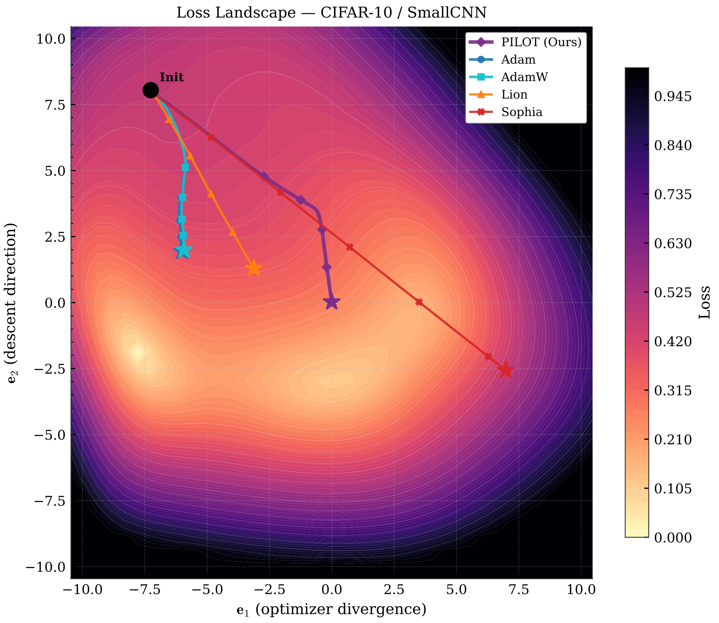
Experiments on FashionMNIST and CIFAR-10 show that PILOT consistently achieves the highest accuracy among the evaluated optimizers across convolutional settings. On the CNN architecture, PILOT reaches 94.13% on FashionMNIST and 81.94% on CIFAR-10. On ResNet-18, it further improves performance, reaching 95.71% on FashionMNIST and 93.42% on CIFAR-10.
Most optimizers like Adam apply the same update formula from the first step to the last. But training dynamics change — early on, gradients are noisy and inconsistent; later, they stabilize as the model approaches a minimum. PILOT adapts its update rule on the fly by reading a simple signal from the gradients themselves.
At each step, PILOT measures how much the current gradient agrees with the previous one using cosine similarity. This raw signal is smoothed into a running score:
When \(\rho\) is high, gradients are pointing in the same direction — the landscape is smooth and the optimizer can be aggressive. When \(\rho\) is low or negative, the landscape is noisy or unstable, and the optimizer should be more cautious.
The signal \(\rho\) is fed through a small learned polynomial to produce three control knobs:
The entire policy has only \(3(d+1)\) learnable coefficients, where \(d\) is the polynomial degree — typically 9 numbers for a quadratic policy. These are initialized so that PILOT starts as standard Adam and learns to deviate.
The three knobs reshape the update rule. First, a blended direction is formed:
Then the parameter update applies sign compression and variance scaling controlled by the policy:
Setting \(p_m=1\), \(p_v=0.5\), \(p_s=0\) recovers Adam exactly. Setting \(p_s=1\), \(p_v=0\) gives a pure sign update. PILOT interpolates continuously between these extremes.
After each step, the next mini-batch gradient reveals whether the policy's choice helped. PILOT uses a one-step analytic meta-gradient to update the polynomial coefficients — no autograd graph, no second-order methods, no offline meta-training. The policy learns alongside the model at negligible cost.
For the full derivation and ablation studies, see the paper.
| Dataset | Optimizer | Accuracy (%) |
|---|---|---|
| FashionMNIST | Adam | 93.28 |
| FashionMNIST | AdamW | 93.22 |
| FashionMNIST | Lion | 92.91 |
| FashionMNIST | Sophia | 89.14 |
| FashionMNIST | AdaBelief | 93.66 |
| FashionMNIST | PILOT (Ours) | 94.13 |
| CIFAR-10 | Adam | 79.91 |
| CIFAR-10 | AdamW | 79.74 |
| CIFAR-10 | Lion | 80.87 |
| CIFAR-10 | Sophia | 76.46 |
| CIFAR-10 | PILOT (Ours) | 81.94 |
| Dataset | Optimizer | Accuracy (%) |
|---|---|---|
| FashionMNIST | Adam | 95.00 |
| FashionMNIST | AdamW | 95.19 |
| FashionMNIST | Lion | 95.09 |
| FashionMNIST | Sophia | 95.09 |
| FashionMNIST | AdaBelief | 95.33 |
| FashionMNIST | PILOT (Ours) | 95.71 |
| CIFAR-10 | Adam | 93.18 |
| CIFAR-10 | AdamW | 92.90 |
| CIFAR-10 | Lion | 92.71 |
| CIFAR-10 | Sophia | 91.76 |
| CIFAR-10 | PILOT (Ours) | 93.42 |
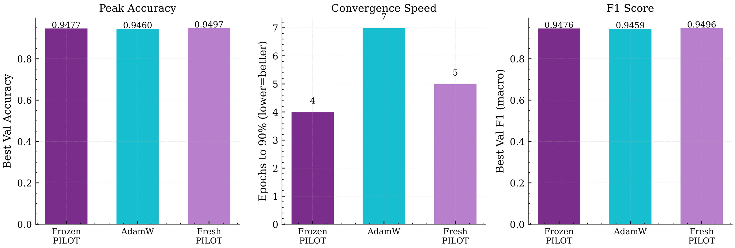
A natural question is whether the learned policy captures optimization dynamics that generalize across datasets, or whether the polynomial coefficients are specific to the task on which they were learned. To test this, a policy is first trained on CIFAR-10 using ResNet-18, then frozen and applied to FashionMNIST with a fresh model initialization.
The frozen policy outperforms AdamW in accuracy, F1 score, and convergence speed, reaching 90% validation accuracy in 4 epochs compared with 7 for AdamW. The fresh PILOT variant achieves the strongest final accuracy (94.97%) through additional target-specific adaptation, but the gap relative to the frozen variant is small (0.20 percentage points). This suggests that most of the policy's benefit is already captured by the source-task coefficients, and that the learned polynomial encodes broadly applicable optimization dynamics rather than dataset-specific patterns.
pip install pilot-optimizer
from pilot import PILOT

optimizer = PILOT(
    model.parameters(),
    lr=1e-3,
    betas=(0.9, 0.999),
    weight_decay=1e-4,
    gamma=0.95,        # smoothing for agreement signal
    eta_phi=0.01,      # policy learning rate
    degree=2           # polynomial degree
)

for batch in dataloader:
    loss = criterion(model(x), y)
    optimizer.zero_grad()
    loss.backward()
    optimizer.step()
@misc{altuuaim2026pilotpolicyinformedlearnedoptimization,
      title={PILOT: Policy-Informed Learned Optimization for Adaptive Deep Network Training},
      author={Sattam Altuuaim and Lama Ayash and Muhammad Mubashar and Naeemullah Khan},
      year={2026},
      eprint={2605.24570},
      archivePrefix={arXiv},
      primaryClass={cs.LG},
      url={https://arxiv.org/abs/2605.24570},
}